
Seasonal prediction of summer Arctic sea ice extent
Since 1979, several organisations have provided satellite data giving information about the Arctic sea ice extent (SIE). The Arctic SIE is defined as the area covered by a significant amount of sea ice, with a threshold of 15% sea ice concentration (EUMETSAT). With these observations, it's possible to produce time series representing the evolution of the Arctic SIE almost over the last 50 years. As shown by the regression line illustrating the global trend, the SIE decrease has been sharp since the 80’s, with several underlying implications for climate and human life.
This website aims to give an overview of seasonal prediction of summer Arctic SIE. Firstly, we explain why SIE prediction has become an important scientific research field in recent years. Then, the mechanisms on which the seasonal prediction is based are reviewed. Lastly, we illustrate the different steps to produce a forecast of SIE for September 2022, based on observations until May 2022.

September Arctic SIE observed and trend line associated
© Sergei Starostin


Importance of Arctic sea ice prediction
Sea ice is frozen ocean water, and it appears in both Arctic and Antarctic oceans. It forms during winter months and disappears during summer months (9). Arctic sea ice reaches its minimum extent each September. The following video shows the annual September SIE since 1979. The Arctic SIE decreases at a rate of 13 % per decade, and the lowest extents recorded were reached in September 2007 and 2012 (1,6,7).
Sea ice is a critical component of the Earth system through its influence on climate (1,4) and human activities (1,11). In the last few years, the interest for seasonal forecasting of Arctic SIE has increased a lot, more especially when the massive reduction occurred in September 2007. Indeed, the decrease in SIE opens new opportunities for scientific and human activities in the Arctic regions (1).
The impact of sea ice on the climate is mainly due to the albedo. Sea ice has a mean albedo of 80 % whereas, without sea ice, water surface will absorb 90 % of the sunlight (9). So, areas covered by sea ice don’t absorb much solar energy, resulting in relatively cool surface temperatures. If sea ice melts because of increasing global temperature, there will be less and less bright surfaces to reflect the sun radiation back to space. Then, a positive ice - albedo feedback, triggered by anthropogenics activities, will occur. As the polar regions are the most sensitive areas to climate change, even a small increase in temperature will lead to a strong warming over time (8).
Ocean dynamics is also affected by sea ice. Indeed, water below sea ice is saltier than the surrounding water. This difference in salt concentration contributes to the ocean’s global “conveyor-belt” circulation. The cold and dense water sinks to the ocean bottom towards the equator, while warm water circulates from the equator towards the poles. Changes in SIE can lead to changes in the ocean circulation pattern, thereby leading to changes in global climate (8).
The regional change in Arctic SIE affects weather and climate in low latitudes. The sea ice cover at the end of the summer can be linked to some winter patterns like the North Atlantic Oscillation and blocking in Western Europe. As a result, it could be useful for mid-latitudes areas to forecast accurately the SIE (1).
The reduction of SIE could allow for an increase in human activities in the Arctic region such as tourism, fishing, navigation or extraction of oil and minerals. Consequently, more accurate forecast would become important to ensure the proper functioning of human activities. Meanwhile, better knowledge of SIE and how it evolves on a seasonal timescale will allow for better planning, thus leading to a reduction in costs and risks of human activities (1).
SIE prediction is therefore useful for many climate observations and human activities in low and mid-latitude areas. Accurate forecasts will lead to a better understanding of climate system and its changes, which is critical in the current context of climate crisis. Finally, better knowledge of the evolution of Arctic SIE can help to find mitigation solutions.
Arctic sea ice minimum since 1979 (corresponding to September extent), based on satellite observations (7)
How to predict sea ice extent?
Forecasting sea ice cover in the Arctic is quite tricky, due to much less abundant observations in the Arctic than in other locations and thus less accurate knowledge of initial conditions (1). Despite this, the scientific community believes that it is possible to predict summer SIE based on sea ice conditions a few months earlier. Indeed, for example, Holland et al. (2011) and Kauker et al. (2009) have shown that winter sea ice thickness in the Arctic represents a good source of predictability for summer ice extent (1). The major source of predictability for seasonal forecasts of Arctic sea ice cover is anomaly persistence. Persistence is defined as the time it takes for a time series to become decorrelated from itself (2). In other words, persistence can be defined as the time required for the anomaly to return to climatological values (5). Indeed, it appears that SIE anomalies tend to last for several months so it can be a source of seasonal predictability. Thus, based on the SIE in May for instance, the persistence of the anomaly could predict the SIE during the annual mean cover minimum in September.
Sea ice predictability can be based on anomaly persistence of several variables: ice thickness, sea ice volume, concentration and area. It is important to specify that depending on the variable used for the forecast, the time scales of persistence can differ (4). Thus, sea ice exhibits significant memory associated with the persistence of anomalies on varying temporal scales. It has been observed that the surface properties of Arctic sea ice possess persistence ranging from 1 to 5 months. Regarding the total volume of sea ice, studies tend to show that the persistence can last for periods ranging from 2 to 4 years. For the persistence of sea ice surface, it depends on the season (2). It has also been shown that the persistence of sea ice thickness and sea ice volume is much longer than the persistence of its concentration and area (4). It can be explained by the fact that a thicker ice sheet will have a better resistance to summer melting than a thinner ice sheet (3).
There are also other sources of predictability, which can be divided into 2 categories: mechanisms related to the sea ice itself and mechanisms related to other components such as the atmosphere or the ocean (2). The source of predictability based on the atmosphere is limited beyond 7 to 10 days for predicting concentration, depth, and movement of Arctic sea ice (10). Hence, at this level, the atmosphere doesn't represent a source of seasonal predictability. By contrast, the ocean represents an important source of predictability because ocean anomalies tend to persist over time and can have significant regional impacts (10).
Another source of predictability is re-emergence, i.e. the possibility for some sea ice anomalies to reappear, thus extending the limit of sea ice predictability. In other words, the anomaly information is recorded in one or more variables differing from ice extent, and a re-emergence mechanism for a given sea ice variable relies on the persistence of another variable (4).
Finally, another source of predictability is the feedback of albedo and ocean heat uptake. It can be explained as a reemergence mechanism. The principle is the following: when solar radiation intensifies and temperature increases in spring, the ice melts, causing therefore a decrease in albedo which further intensifies the ice melting. It induces the formation of open water areas that gradually expand with the increase in temperature during the summer. These open water areas absorb a large amount of energy which further increases the energy storage in the system. Therefore, if an open water area develops earlier than usual during spring, the energy uptake by the system will be greater during the summer season and thus the open water areas will last longer than usual. Finally, as spring and summer energy uptake increases, fall ice growth is delayed because it takes longer for the ocean to lose the absorbed heat. The initial feedback anomalies in albedo and ocean heat uptake have several possible sources. Indeed, the onset of spring melt or the melt fraction of the top of sea ice may be a source of predictability because of their effects on surface albedo. Both these processes depend on temperature anomalies and snowfall anomalies (10).
To sum up, there are several sources of predictability of Arctic sea ice cover. Predictability in this location is particularly challenging due to the limited number of observations and the large number of interactions between the different components. However, the persistence of anomalies on seasonal time scales makes forecasting possible if we have a good knowledge of the initial conditions. For that reason, the forecast of September SIE, described below, is based on anomaly persistence.
-
Predictability: Extent to which the distribution of future states of a certain variable, conditioned either on knowledge of observations at the initial time or on knowledge of future forcings, is different from the climatological distribution (5).
-
Climatological distribution: A climatological distribution is the statistical distribution of state at verification time, unconditional on observations. The climatological distribution describes the set of future states that are compatible with the system’s state history (5).
-
Threat score: It measures the fraction of observed and/or forecast events that were correctly predicted.
-
Hit rate: It calculates the rate of forecasted events that were well predicted.
-
False alarm rate: It indicates the proportion of observed "no" events that were forecasted as events that happened.
-
False alarm ratio: It indicates the proportion of events predicted to happen that actually didn't occur.
-
Bias: It measures the ratio of the frequency of forecast events to the frequency of observed events.
September Arctic sea ice forecast
Statistical forecasting system
It’s now time to produce a retrospective forecast of September SIE. As said earlier, the anomaly persistence is larger for SIE calculated from its volume and thickness than using the SIE records. Given these elements, the data used for the anomaly persistence forecast are the sea ice volume and thickness (both coming from PIOMAS) to approximate the SIE. We have divided the volume by the thickness to obtain a value that accounts for the sea ice extent. Those two parameters are derived from PIOMAS model based on satellite observations.
Considering that a forecast should be expressed as a probability density function (pdf), it’s needed to consider that the pdf for each year will be a gaussian random variable N(µ, σ²).
The forecast (µ) is made this way: the September SIE for a given year is calculated as the sum of the mean September SIE from 1979 to the previous year and the mean anomaly of SIE ranging from October to May preceding the forecast. The anomaly corresponds to the SIE value to which the mean SIE value is subtracted. A standard deviation (σ) is associated to the forecast to reflect uncertainty in the model and in the initial conditions (the sea ice thickness, volume and extents observations).
The forecast is then compared to satellite observations of SIE coming from EUMETSAT.
The code used to perform the forecast and obtain the results presented below is available here.
In some cases, forecasts don’t really fit the observations made in the same period. Several reasons could explain this, but it generally comes from the simplicity of the model, which induces inaccuracies in the results. To remedy these imprecisions, it’s important to proceed to some post-processing corrections, which of course don’t enhance the model itself but improve the forecast results.
In our case, we clearly noticed a trend bias: the decreasing trend of sea ice extent wasn’t well taken into account by the model. As a result, forecasts for recent years overestimated the sea ice extent. This bias has been removed by detrending the forecasts and adding the trend of the observations. Of course this model, due to its simplicity, is not going to give the exact forecast for the September SIE but it represents the first step on the road of a correct prediction.
This figure shows the final predicted SIE in September, based on anomaly persistence of sea ice volume and thickness and with the bias trend removed. We observe that the forecasts aren't always corresponding correctly to the observations, especially for the low peaks in 2007 and 2012. But the forecasts aren't particularly inaccurate, illustrating that the method used isn't irrelevant, even if it could be improved.
The forecasted SIE for September 2022 is 4 905 785 km².
Once the September SIE has been forecasted, it is interesting to make sense of it by comparing it to predefined values, called “events”. Here, the event is defined as follows: “September sea ice extent is less than previous year”. For each year, the probability that the event happens can be calculated. In other words, the probability that the forecasted value is less than the previous year sea ice extent is calculated. Then, the probability based on the forecast is compared to the occurrence of the event in the observations.
The figure shows the events which were correctly predicted (high probability and green) and the ones where for which the forecast was not accurate (i.e. high probability and red). Our forecast tends to predict event occurrence with extremes probabilities, i.e. close to 0 or to 1.
The probability to reach a September SIE lower in 2022 than in 2021 is 96.7 %. This probability is very high because our forecast system is overconfident.
To check the matching between the frequency of occurrence of the event and the probability previously calculated, we proceed to a verification. This operation takes into account the number of years for which we calculate the probability of event occurrence, the probability of event occurrence itself and the observation of that event. The first verification score used is the Brier’s score (BS) and the Brier’s skill score (BSS), which give an idea of accuracy with an index between 0 and 1. The BSS takes the climatology into account (which corresponds to a BS of reference) to evaluate the performances of the forecast compared to climatological prevision. The formula are the following:
The best forecast is characterized by a BS closest to 0. Here, it is equal to 0.17. The best forecast has also a BS significantly different from the BS of reference, which leads to a BSS close to 1. Here, the BS of reference is equal to 0.25, resulting in a BSS equal to 0.32. Consequently, the forecast could be greatly improved, but our model still gives better results than a forecast based on climatology.
In addition to this Brier’s score, many other indexes can be used to improve the quality of the verification.
Using the contingency table below, we have calculated some scores to evaluate the quality of the event forecast. The threat score and hit rate are best when they are equal to 100 %. In this situation they are respectively equal to 69.0 % and 87.0 % which means that the forecast is quite accurate, even if it could be better. False alarm ratio and false alarm rate both focus on the forecasted events that actually didn't happen, and are ideally equal to 0 %. Here, we obtained values of 23.1 % and 33.3 % respectively, meaning again a not so bad forecast. Finally the bias is perfect when it's equal to 1. Our 1.13 value indicates nearly no bias variation.
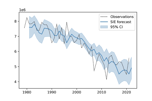
September Arctic SIE extent observed (dashed line), and forecasted with the corresponding 95% confidence interval (blue)
Forecast correction
Retrospective probabilistic forecast of the event

Probability of event occurrence for volume based forecast of SIE. The red bars show years for which the event didn't happen while the green ones show year for which the event happend. The grey bar correspond to 2022 forecast.
Verification

Contingency table
Blockley, E. W., & Peterson, K. A. (2018). Improving Met Office seasonal predictions of Arctic sea ice using assimilation of CryoSat-2 thickness. The Cryosphere, 12(11), 3419-3438. (1)
Chevallier, M., Massonnet, F., Goessling, H., Guémas, V., & Jung, T. (2019). The role of sea ice in sub-seasonal predictability. In Sub-seasonal to seasonal prediction (pp. 201-221). Elsevier. (2)
Chevallier, M., & Salas-Mélia, D. (2012). The role of sea ice thickness distribution in the Arctic sea ice potential predictability: A diagnostic approach with a coupled GCM. Journal of Climate, 25(8), 3025-3038. (3)
Guemas, V., Blanchard‐Wrigglesworth, E., Chevallier, M., Day, J. J., Déqué, M., Doblas‐Reyes, F. J., ... & Tietsche, S. (2016). A review on Arctic sea‐ice predictability and prediction on seasonal to decadal time‐scales. Quarterly Journal of the Royal Meteorological Society, 142(695), 546-561. (4)
Massonnet F. (2022). LPHYS2268 Course notes (5)
Msadek, R., Vecchi, G. A., Winton, M., & Gudgel, R. G. (2014). Importance of initial conditions in seasonal predictions of Arctic sea ice extent. Geophysical Research Letters, 41(14), 5208-5215. (6)
NASA. (s.d.). Arctic Sea Ice Extent. Climate.nasa.gov. https://climate.nasa.gov/vital-signs/arctic-sea-ice/ (7)
NSIDC. (s.d.). All About Sea Ice. (2020, 3 April). National Snow and Ice Data Center. https://nsidc.org/cryosphere/seaice/index.html (8)
NSIDC. (s.d.). Quick Facts on Arctic Sea Ice. National Snow and Ice Data Center. https://nsidc.org/cryosphere/quickfacts/seaice.html (9)
Serreze, M. C., & Meier, W. N. (2019). The Arctic's sea ice cover: trends, variability, predictability, and comparisons to the Antarctic. Annals of the New York Academy of Sciences, 1436(1), 36-53. (10)
Zampieri, L., Goessling, H. F., & Jung, T. (2018). Bright prospects for Arctic sea ice prediction on subseasonal time scales. Geophysical Research Letters, 45(18), 9731-9738. (11)